mpl – Convert templates to plots

This module provides the classes to convert test results to plots using matplotlib.pyplot.

MplPlot objects take as input PlotTemplate containing curves (CurveElements) classified by sub-plots (SubPlotElements).

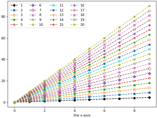
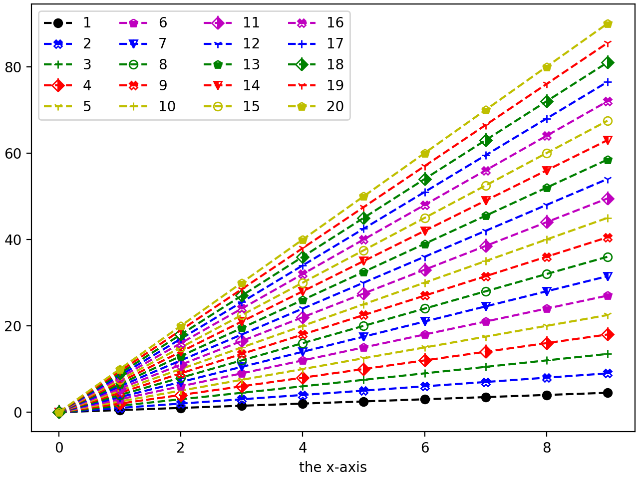
The format, or rendering, of the plot can be set using the rcParams but also some predefined parameters on which the class cycle like colors, markers shape and filling.

By default the first color is black and is used only once: it is excluded from the cycle on colors. It is typically reserved for the reference but can be reused if the first index is used for another curve.

Plots can be obtained with the following for example:

>>> import numpy as np
>>> from valjean.javert.templates import (PlotTemplate, CurveElements,
...                                       SubPlotElements)
>>> bins = (np.array(np.arange(10)),)
>>> lcurves = [CurveElements(values=bins[0]*0.5*(icurve+1), bins=bins,
...                          legend=str(icurve+1), index=icurve)
...            for icurve in range(20)]
>>> pltit = PlotTemplate(subplots=[SubPlotElements(
...     curves=lcurves, axnames=('the x-axis', ''), ptype='1D')])
>>> from valjean.javert.mpl import MplPlot
>>> mplplt = MplPlot(pltit)
>>> fig, _ = mplplt.draw()

(Source code, png, hires.png, pdf)

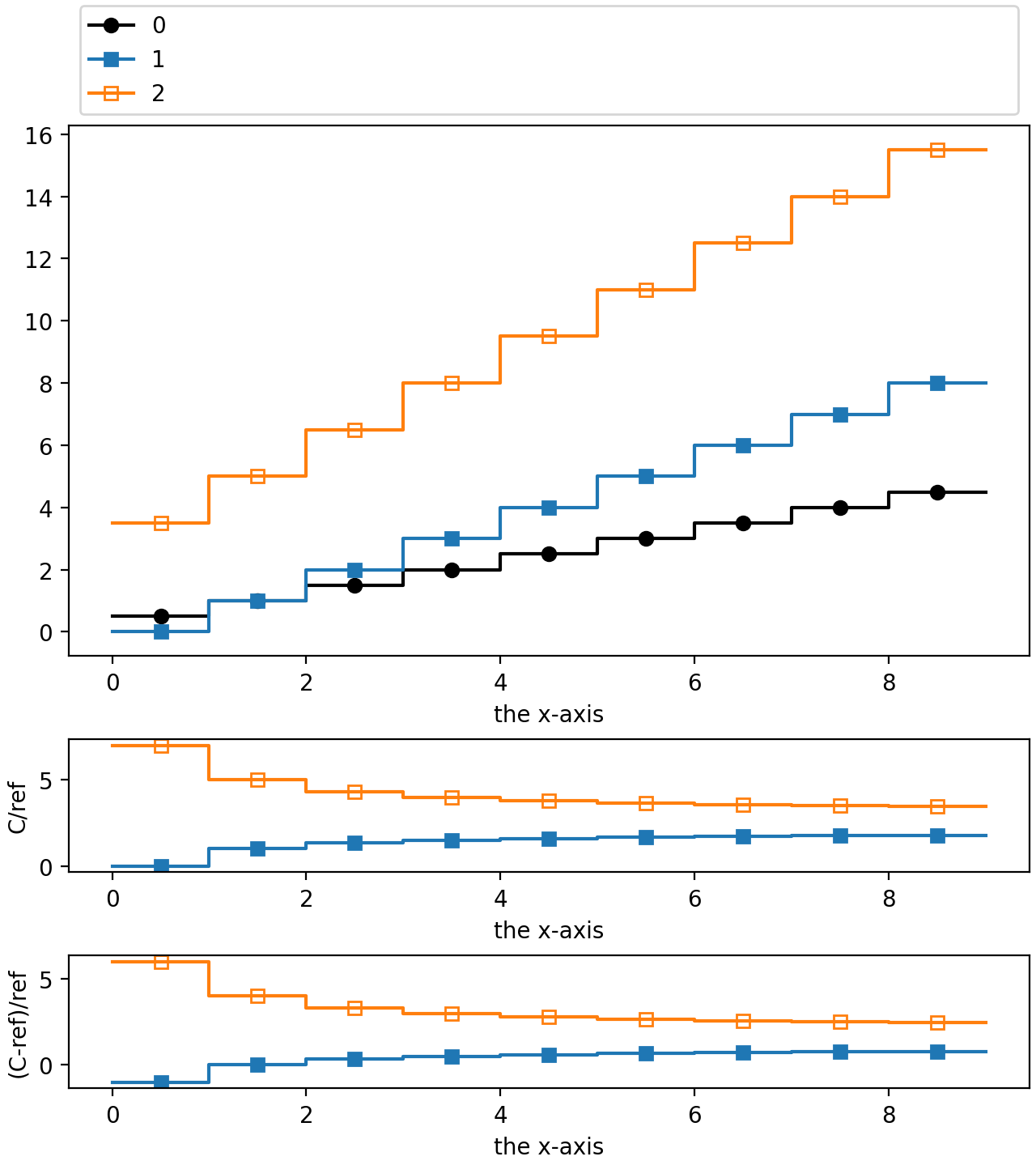
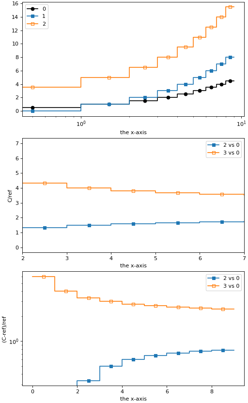
Additional subplots can be drawn if required. The style of the curves is fixed by the index (see CurveElements).

>>> import numpy as np
>>> from valjean.javert.templates import (PlotTemplate, CurveElements,
...                                       SubPlotElements)
>>> bins = (np.array(np.arange(10)),)
>>> lcurves1 = []
>>> for icurve in range(3):
...     lcurves1.append(CurveElements(
...         values=bins[0][1:]*0.5*(icurve+1) + icurve*(-1)**(icurve),
...         bins=bins, legend=str(icurve), index=icurve))
>>> sbpe1 = SubPlotElements(curves=lcurves1, axnames=('the x-axis', ''))
>>> lcurves2 = []
>>> for icurve in range(1, 3):
...     lcurves2.append(CurveElements(
...         values=lcurves1[icurve].values/lcurves1[0].values, bins=bins,
...         legend=str(icurve+1), index=icurve))
>>> sbpe2 = SubPlotElements(curves=lcurves2,
...                         axnames=('the x-axis', 'C/ref'))
>>> lcurves3 = []
>>> for icurve in range(1, 3):
...     lcurves3.append(CurveElements(
...         values=((lcurves1[icurve].values-lcurves1[0].values)
...                 /lcurves1[0].values),
...         bins=bins, legend=str(icurve+1), index=icurve))
>>> sbpe3 = SubPlotElements(curves=lcurves3,
...                         axnames=('the x-axis', '(C-ref)/ref'))
>>> pltit = PlotTemplate(subplots=[sbpe1, sbpe2, sbpe3])
>>> from valjean.javert.mpl import MplPlot
>>> mplplt = MplPlot(pltit)
>>> fig, _ = mplplt.draw()

(Source code, png, hires.png, pdf)

These examples also show the default style of the plots.

Style setup

Some style parameters are available in the object MplStyle: general style, colors of markers and lines (expected to be the same for the same curve), shapes and fills of markers. Legend keyword arguments can also be given.

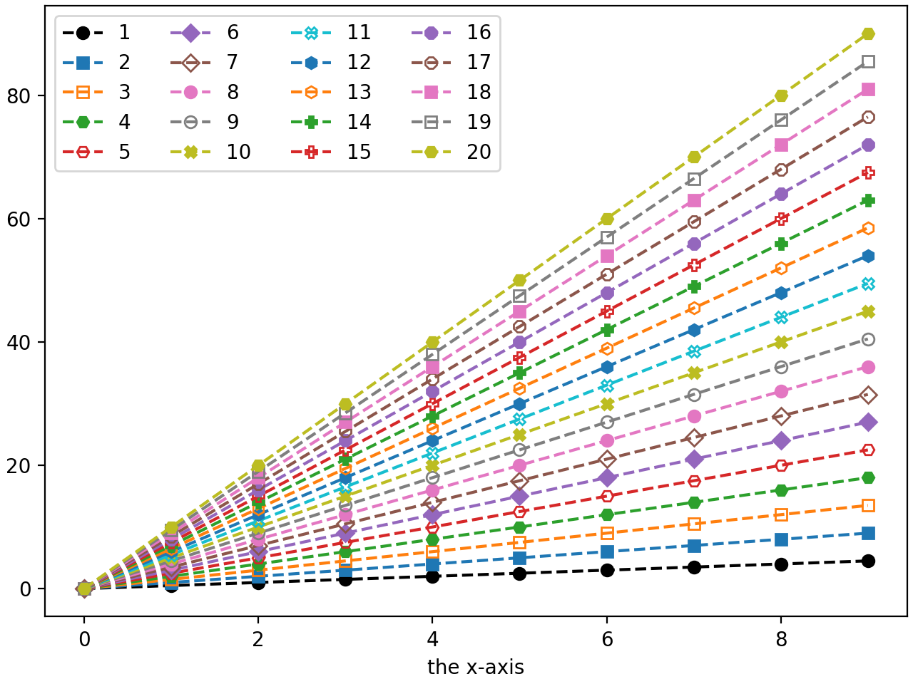
General style

It is possible to change the general style of plots using a predefined one or to use different markers. The predefined styles can be seen in matplotlib styles or be obtained thanks to

>>> import matplotlib.pyplot as plt  
>>> print(plt.style.available)  

For example, we can have:

>>> import numpy as np
>>> from valjean.javert.templates import (PlotTemplate, CurveElements,
...                                       SubPlotElements)
>>> bins = (np.array(np.arange(10)),)
>>> lcurves = []
>>> for icurve in range(20):
...     lcurves.append(CurveElements(values=bins[0]*0.5*(icurve+1),
...                                  bins=bins, legend=str(icurve+1),
...                                  index=icurve))
>>> sbpe = SubPlotElements(curves=lcurves, axnames=['the x-axis', ''])
>>> pltit = PlotTemplate(subplots=[sbpe])
>>> from valjean.javert.mpl import MplPlot, MplStyle
>>> mplplt = MplPlot(pltit, style=MplStyle(style='Solarize_Light2'))
>>> fig, _ = mplplt.draw()

(Source code, png, hires.png, pdf)

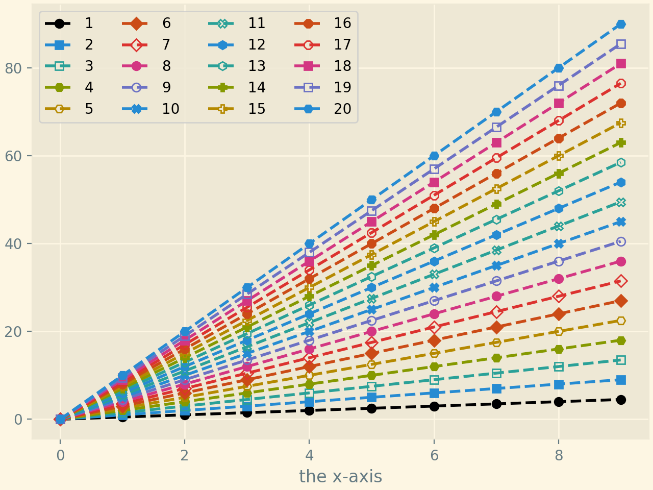
Colors and markers

Colors and markers can also be changed directly:

>>> import numpy as np
>>> from valjean.javert.templates import (PlotTemplate, CurveElements,
...                                       SubPlotElements)
>>> bins = [np.array(np.arange(10))]
>>> lcurves = []
>>> for icurve in range(20):
...     lcurves.append(CurveElements(values=bins[0]*0.5*(icurve+1),
...                                  bins=bins, legend=str(icurve+1),
...                                  index=icurve))
>>> sbpe = SubPlotElements(curves=lcurves, axnames=['the x-axis', ''])
>>> pltit = PlotTemplate(subplots=[sbpe])
>>> from valjean.javert.mpl import MplPlot, MplStyle
>>> style = MplStyle(colors=['b', 'g', 'r', 'y', 'm'],
...                  mshape=['X', '+', 'D', '1', 'p', 'v', 'o'],
...                  mfill=['top', 'full', 'right', 'none', 'bottom',
...                         'left', 'none'])
>>> mplplt = MplPlot(pltit , style=style)
>>> fig, _ = mplplt.draw()

(Source code, png, hires.png, pdf)

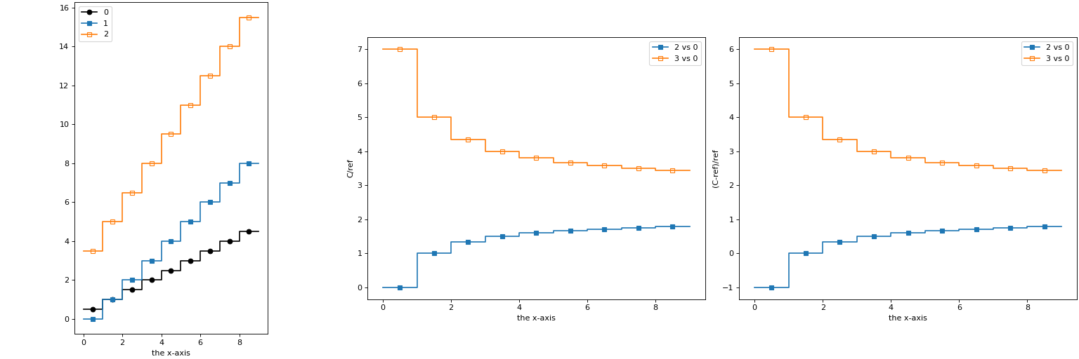
Legends

By default the legend is represented on all panels at the location matplotlib.pyplot determines like in plot 3 panels.

If you would prefer to get only one legend for all panels, the suppress_legends argument in PlotTemplate should be used. In that case, only fine for 1D plots, the legend will be placed on the largest panel by default.

In the style any keyword argument accepted by matplotlib can be given to modify for example the legend position. This is can be found in the legend documentation.

The next example show the plot 3 panels with only one legend which position and shape have been modified.

>>> import numpy as np
>>> from valjean.javert.templates import (PlotTemplate, CurveElements,
...                                       SubPlotElements)
>>> bins = [np.array(np.arange(10))]
>>> lcurves1 = []
>>> for icurve in range(3):
...     lcurves1.append(CurveElements(
...         values=bins[0][1:]*0.5*(icurve+1) + icurve*(-1)**(icurve),
...         bins=bins, legend=str(icurve), index=icurve))
>>> sbpe1 = SubPlotElements(curves=lcurves1, axnames=['the x-axis', ''])
>>> lcurves2 = []
>>> for icurve in range(1, 3):
...     lcurves2.append(CurveElements(
...         values=lcurves1[icurve].values/lcurves1[0].values,
...         bins=bins, legend=str(icurve+1)+' vs 0', index=icurve))
>>> sbpe2 = SubPlotElements(curves=lcurves2,
...                         axnames=['the x-axis', 'C/ref'])
>>> lcurves3 = []
>>> for icurve in range(1, 3):
...     lcurves3.append(CurveElements(
...         values=((lcurves1[icurve].values-lcurves1[0].values)
...                 /lcurves1[0].values),
...         bins=bins, legend=str(icurve+1)+' vs 0', index=icurve))
>>> sbpe3 = SubPlotElements(curves=lcurves3,
...                         axnames=['the x-axis', '(C-ref)/ref'])
>>> pltit = PlotTemplate(subplots=[sbpe1, sbpe2, sbpe3],
...                      suppress_legends=True)
>>> from valjean.javert.mpl import MplPlot, MplStyle
>>> style = MplStyle(legends={'loc': 3, 'bbox_to_anchor': (0., 1., 1, 1),
...                           'mode': 'expand'})
>>> mplplt = MplPlot(pltit, style=style)
>>> fig, _ = mplplt.draw()

(Source code, png, hires.png, pdf)

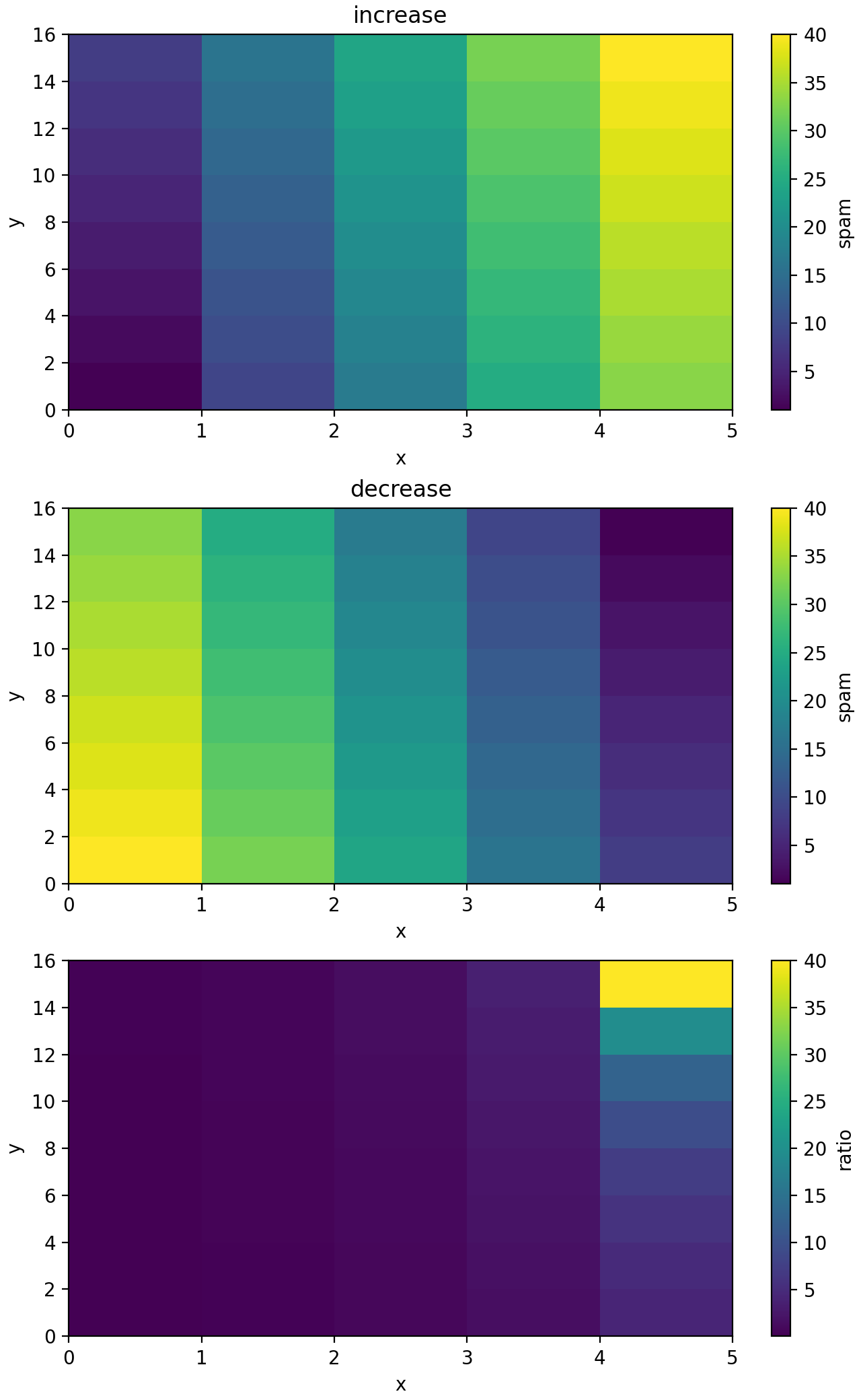
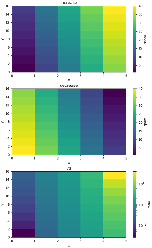
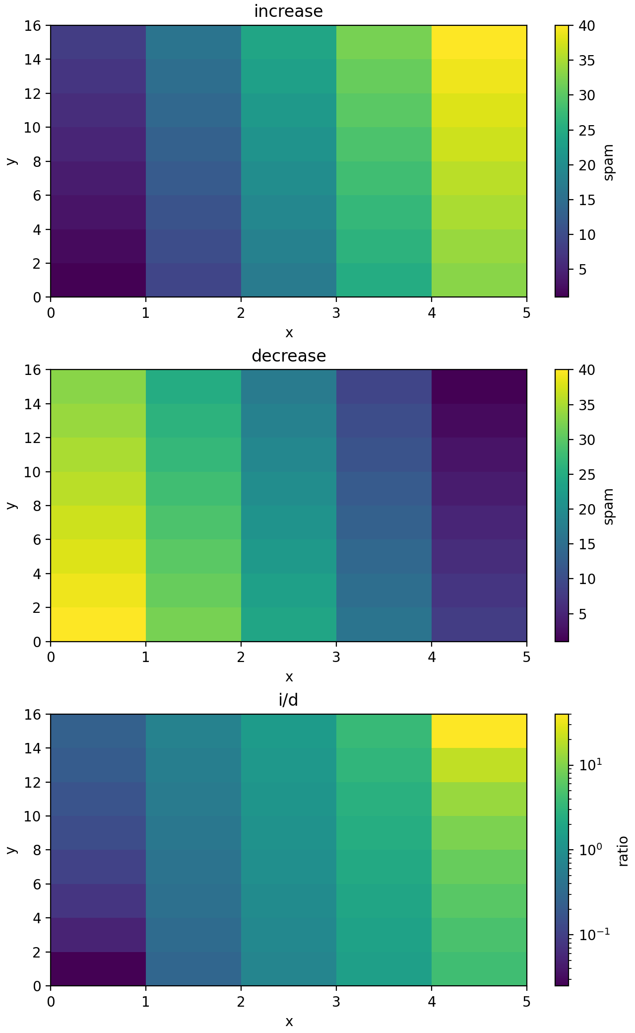
2D plots

2D plots are also done via the class MplPlot. The plot type ptype in PlotTemplate should be '2D'. The principle is the same as for 1D plots. Three axes are expected. Each curve has its own plot, no superposition is done, so one subplot is expected to contain only one curve. Each subplot can then have its own properties.

The colorbar axis label is set using the third axis name.

There is no real legend, so legend is used as title of each plot.

The index is currently not used.

>>> from collections import OrderedDict
>>> import numpy as np
>>> from valjean.javert.templates import (PlotTemplate, CurveElements,
...                                       SubPlotElements)
>>> bins = [np.arange(6), np.arange(17, step=2)]
>>> axnames = ['x', 'y']
>>> incv = np.arange(1, 41).reshape(5, 8)
>>> decv = np.arange(1, 41)[::-1].reshape(5, 8)
>>> lsplts = []
>>> lsplts.append(SubPlotElements(
...     curves=[CurveElements(
...         values=incv, bins=bins, legend='increase', index=0)],
...     axnames=['x', 'y', 'spam'], ptype='2D'))
>>> lsplts.append(SubPlotElements(
...     curves=[CurveElements(
...         values=decv, bins=bins, legend='decrease', index=0)],
...     axnames=['x', 'y', 'spam'], ptype='2D'))
>>> lsplts.append(SubPlotElements(
...     curves=[CurveElements(
...         values=incv/decv, bins=bins, legend='', index=1)],
...     axnames=['x', 'y', 'ratio'], ptype='2D'))
>>> pltnd = PlotTemplate(subplots=lsplts, small_subplots=False)
>>> from valjean.javert import mpl
>>> mplplt = mpl.MplPlot(pltnd)
>>> fig, _ = mplplt.draw()

(Source code, png, hires.png, pdf)

Note

Per default, additional subplots are small ones, it is probably better in 2D case to set the parameter small_subplots to False in the PlotTemplate.

Warning

Requesting more than one curve on a subplot will emit a warning but give unexpected results (typically only one of the 2D plot will be shown).

>>> from collections import OrderedDict
>>> import numpy as np
>>> from valjean.javert.templates import (PlotTemplate, CurveElements,
...                                       SubPlotElements)
>>> bins = [np.arange(6), np.arange(17, step=2)]
>>> axnames = ['x', 'y']
>>> incv = np.arange(1, 41).reshape(5, 8)
>>> decv = np.arange(1, 41)[::-1].reshape(5, 8)
>>> lsplts = []
>>> lsplts.append(SubPlotElements(
...     curves=[CurveElements(values=incv, bins=bins, legend='increase'),
...             CurveElements(values=decv, bins=bins, legend='decrease')],
...     axnames=['x', 'y', 'spam'], ptype='2D'))
>>> lsplts.append(SubPlotElements(
...     curves=[CurveElements(
...         values=incv/decv, bins=bins, legend='', index=1)],
...     axnames=['x', 'y', 'ratio'], ptype='2D'))
>>> pltnd = PlotTemplate(subplots=lsplts)
>>> from valjean.javert import mpl
>>> mplplt = mpl.MplPlot(pltnd)
>>> fig, _ = mplplt.draw()

(Source code, png, hires.png, pdf)

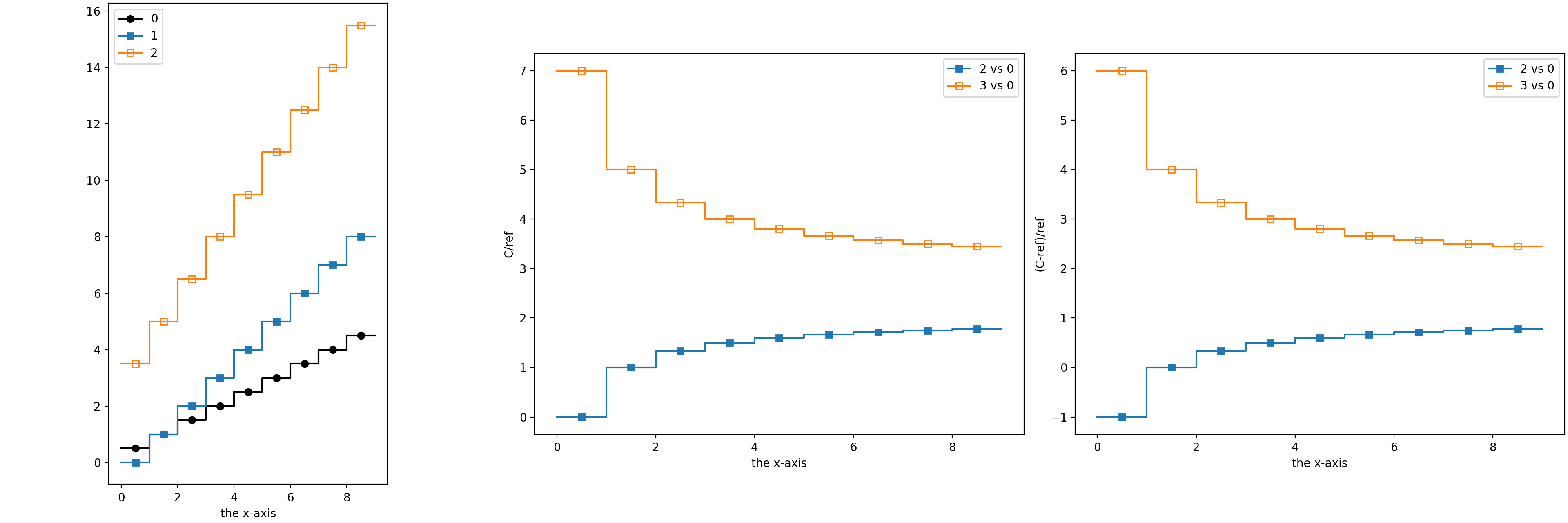
Customization

Some customizations can be done for each subplot with the attributes parameter of SubPlotElements: limits to adapt axes ranges, logarithmic scale or lines.

Using the previous 1D example:

>>> import numpy as np
>>> from valjean.javert.templates import (PlotTemplate, CurveElements,
...                                       SubPlotElements)
>>> bins = [np.array(np.arange(10))]
>>> lcurves1 = [CurveElements(
...     values=bins[0][1:]*0.5*(icurve+1) + icurve*(-1)**(icurve),
...     bins=bins, legend=str(icurve), index=icurve)
...             for icurve in range(3)]
>>> sbpe1 = SubPlotElements(curves=lcurves1, axnames=['the x-axis', ''])
>>> lcurves2 = [CurveElements(
...     values=lcurves1[icurve].values/lcurves1[0].values, bins=bins,
...     legend=str(icurve+1)+' vs 0', index=icurve)
...             for icurve in range(1, 3)]
>>> sbpe2 = SubPlotElements(curves=lcurves2,
...                         axnames=['the x-axis', 'C/ref'])
>>> lcurves3 = [CurveElements(
...     values=((lcurves1[icurve].values-lcurves1[0].values)
...             /lcurves1[0].values),
...     bins=bins, legend=str(icurve+1)+' vs 0', index=icurve)
...             for icurve in range(1, 3)]
>>> sbpe3 = SubPlotElements(curves=lcurves3,
...                         axnames=['the x-axis', '(C-ref)/ref'])
>>> sbpe1.attributes.logx = True
>>> sbpe2.attributes.limits = [(2, 7)]
>>> sbpe3.attributes.logy = True
>>> pltit = PlotTemplate(subplots=[sbpe1, sbpe2, sbpe3],
...                      small_subplots=False)
>>> from valjean.javert.mpl import MplPlot, MplStyle
>>> mplplt = MplPlot(pltit)
>>> fig, _ = mplplt.draw()

(Source code, png, hires.png, pdf)

Customizations specific to the backend, here matplotlib.pyplot, are passed thanks to the backend_kw argument of PlotTemplate. The keywords that are currently supported by the matplotlib.pyplot backend and used in valjean are:

nrows and ncols

These keys should be associated to integers. They determine the number of subplots, in case the PlotTemplate object contains several SubPlotElements. If ncols is given, nrows also has to be given.

figsize

This key should be associated to tuple of floats (width and height in inches) to specify the figure size.

subplot_kw

This key should be associated to a dictionary of keywords that will be passed as-is to matplotlib.pyplot.subplots.

gridspec_kw

This key should be associated to a dictionary to be passed to the grid constructor, see matplotlib.pyplot.subplots and matplotlib.gridspec.GridSpec.

All possible keyword arguments that can be passed to matplotlib.pyplot.subplots are normally supported.

Example is given from the previous 1D one:

>>> import numpy as np
>>> from valjean.javert.templates import (PlotTemplate, CurveElements,
...                                       SubPlotElements)
>>> bins = [np.array(np.arange(10))]
>>> lcurves1 = [CurveElements(
...     values=bins[0][1:]*0.5*(icurve+1) + icurve*(-1)**(icurve),
...     bins=bins, legend=str(icurve), index=icurve)
...             for icurve in range(3)]
>>> sbpe1 = SubPlotElements(curves=lcurves1, axnames=['the x-axis', ''])
>>> lcurves2 = [CurveElements(
...     values=lcurves1[icurve].values/lcurves1[0].values, bins=bins,
...     legend=str(icurve+1)+' vs 0', index=icurve)
...             for icurve in range(1, 3)]
>>> sbpe2 = SubPlotElements(curves=lcurves2,
...                         axnames=['the x-axis', 'C/ref'])
>>> lcurves3 = [CurveElements(
...     values=((lcurves1[icurve].values-lcurves1[0].values)
...             /lcurves1[0].values),
...     bins=bins, legend=str(icurve+1)+' vs 0', index=icurve)
...             for icurve in range(1, 3)]
>>> sbpe3 = SubPlotElements(curves=lcurves3,
...                         axnames=['the x-axis', '(C-ref)/ref'])
>>> pltit = PlotTemplate(subplots=[sbpe1, sbpe2, sbpe3],
...                      small_subplots=False,
...                      backend_kw={'ncols': 3, 'nrows': 1,
...                                  'subplot_kw': {'aspect': 'equal'}})
>>> from valjean.javert.mpl import MplPlot, MplStyle
>>> mplplt = MplPlot(pltit)
>>> fig, _ = mplplt.draw()

(Source code, png, hires.png, pdf)

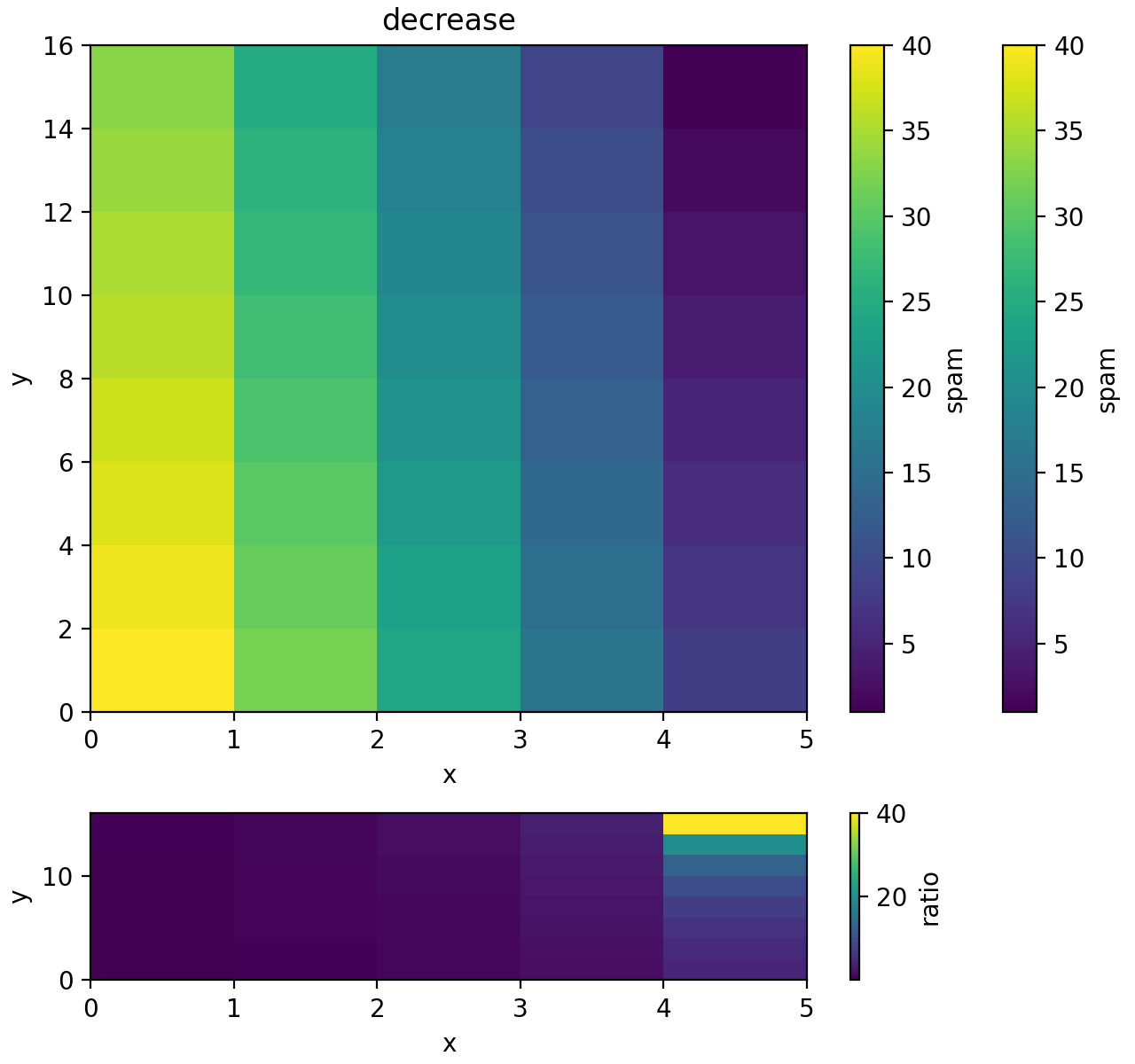
Customization also works on 2D plots. In addition the colorscale and colormap can be put in logarithmic scale.

>>> from collections import OrderedDict
>>> import numpy as np
>>> from valjean.javert.templates import (PlotTemplate, CurveElements,
...                                       SubPlotElements)
>>> bins = [np.arange(6), np.arange(17, step=2)]
>>> axnames = ['x', 'y']
>>> incv = np.arange(1, 41).reshape(5, 8)
>>> decv = np.arange(1, 41)[::-1].reshape(5, 8)
>>> sbp1 = SubPlotElements(
...     curves=[CurveElements(values=incv, bins=bins, legend='increase')],
...     axnames=['x', 'y', 'spam'], ptype='2D')
>>> sbp2 = SubPlotElements(
...     curves=[CurveElements(values=decv, bins=bins, legend='decrease')],
...     axnames=['x', 'y', 'spam'], ptype='2D')
>>> sbp3 = SubPlotElements(
...     curves=[CurveElements(values=incv/decv, bins=bins, legend='i/d')],
...     axnames=['x', 'y', 'ratio'], ptype='2D')
>>> sbp3.attributes.logz = True
>>> pltnd = PlotTemplate(subplots=[sbp1, sbp2, sbp3], small_subplots=False)
>>> from valjean.javert import mpl
>>> mplplt = mpl.MplPlot(pltnd)
>>> fig, _ = mplplt.draw()

(Source code, png, hires.png, pdf)

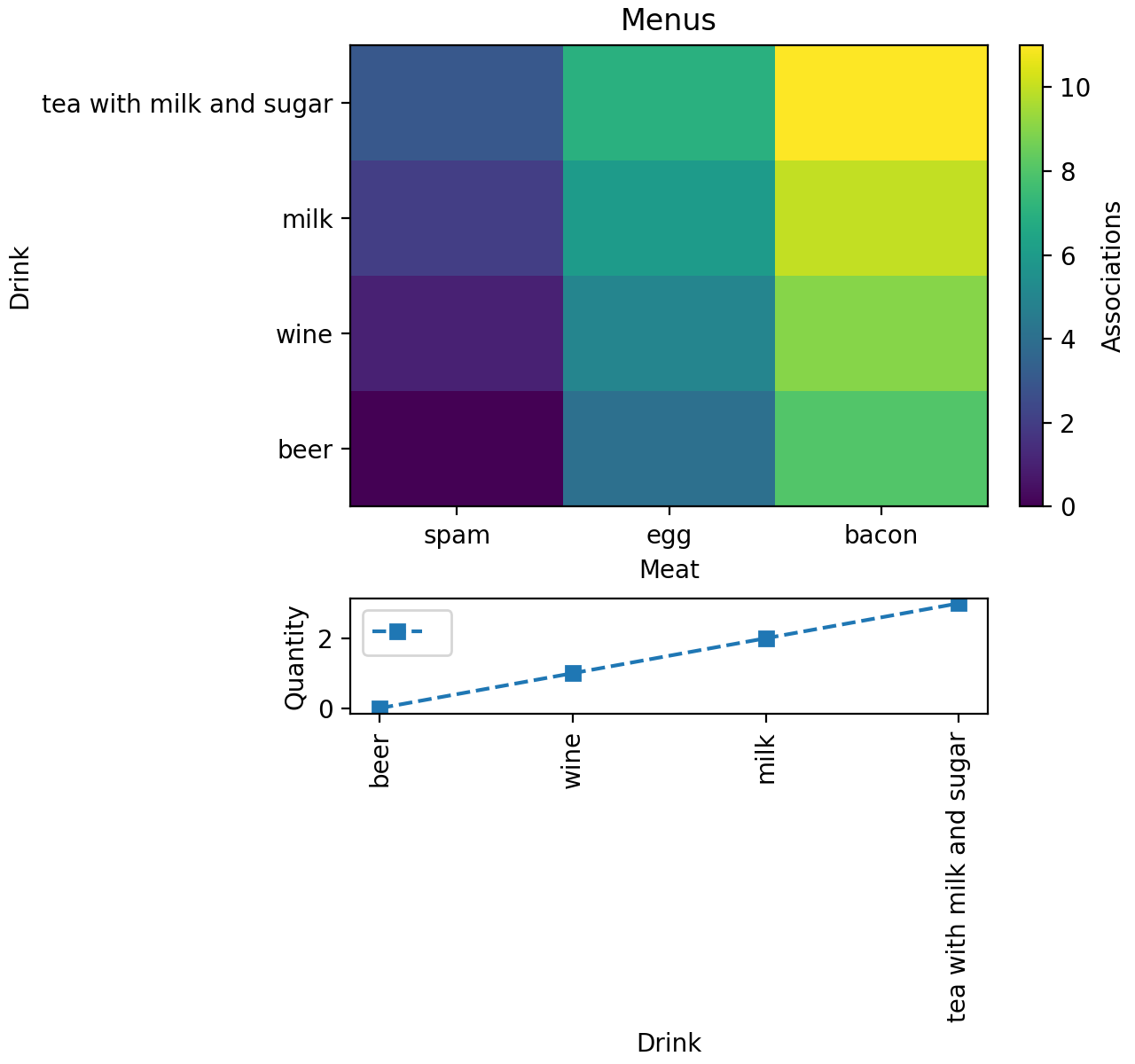
Strings as bins

It is possible to use strings as bins both in 1D and 2D plots. If strings are too long on x-axis they will be represented vertically.

>>> from collections import OrderedDict
>>> import numpy as np
>>> from valjean.javert.templates import (PlotTemplate, CurveElements,
...                                       SubPlotElements)
>>> bins = [np.array(['spam', 'egg', 'bacon']),
...         np.array(['beer', 'wine', 'milk', 'tea with milk and sugar'])]
>>> axnames = ['x', 'y']
>>> v2d = np.arange(12).reshape(3, 4)
>>> v1d = np.arange(4)
>>> lsplts = []
>>> lsplts.append(SubPlotElements(
...     curves=[CurveElements(values=v2d, bins=bins, legend='Menus')],
...     axnames=['Meat', 'Drink', 'Associations'], ptype='2D'))
>>> lsplts.append(SubPlotElements(
...     curves=[CurveElements(
...         values=v1d, bins=bins[1:], legend='', index=1)],
...     axnames=['Drink', 'Quantity'], ptype='1D'))
>>> pltnd = PlotTemplate(subplots=lsplts)
>>> from valjean.javert import mpl
>>> mplplt = mpl.MplPlot(pltnd)
>>> fig, _ = mplplt.draw()

(Source code, png, hires.png, pdf)

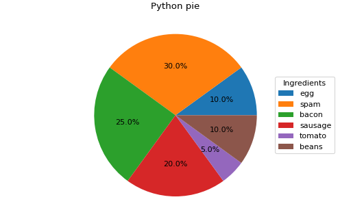
Pie plot

Pie plots can be done if requested. ptype should be equal to ‘pie’. Note that the number of axnames still has to be N dim + 1, so 2. The first one is the title of the plot, the second one the title of the legend. If the second string is empty no title will be given to the legend.

>>> import numpy as np
>>> from valjean.javert.templates import (PlotTemplate, CurveElements,
...                                       SubPlotElements)
>>> ingredients = ['egg', 'spam', 'bacon', 'sausage', 'tomato', 'beans']
>>> proportions = [0.1, 0.3, 0.25, 0.2, 0.05, 0.1]
>>> curve = CurveElements(values=np.array(proportions),
...                       bins=[ingredients], legend='')
>>> sbplt = SubPlotElements(curves=[curve],
...                         axnames=('Python pie', 'Ingredients'),
...                         ptype='pie')
>>> pltpie = PlotTemplate(subplots=[sbplt])
>>> from valjean.javert import mpl
>>> mplplt = mpl.MplPlot(pltpie)
>>> fig, _ = mplplt.draw()

(Source code, png, hires.png, pdf)

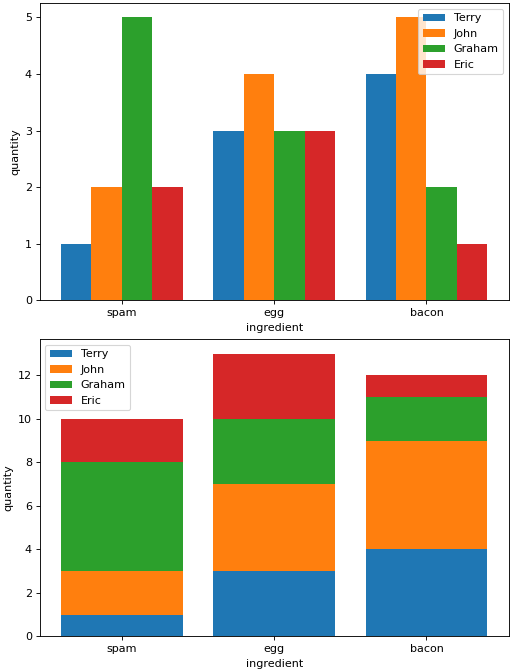
Bar plots

Bar plots can be used here with strings as labels in x-axis, like category plots but no errors are expected here. Two kinds of bar plots are available: side-by-side bars and stacked bars.

>>> import numpy as np
>>> from valjean.javert.templates import (PlotTemplate, CurveElements,
...                                       SubPlotElements)
>>> bins = [np.array(['spam', 'egg', 'bacon'])]
>>> data = [np.array([1, 3, 4]),  np.array([2, 4, 5]),
...         np.array([5, 3, 2]), np.array([2, 3, 1])]
>>> names = ['Terry', 'John' , 'Graham', 'Eric']
>>> lcurves = []
>>> for datum, name in zip(data, names):
...     lcurves.append(CurveElements(values=datum, bins=bins, legend=name))
>>> speb = SubPlotElements(curves=lcurves,
...                        axnames=['ingredient', 'quantity'], ptype='bar')
>>> spebs = SubPlotElements(curves=lcurves,
...                         axnames=['ingredient', 'quantity'],
...                         ptype='barstack')
>>> pltbar = PlotTemplate(subplots=[speb, spebs], small_subplots=False)
>>> from valjean.javert import mpl
>>> mplplt = mpl.MplPlot(pltbar)
>>> fig, _ = mplplt.draw()

(Source code, png, hires.png, pdf)

Module API

class valjean.javert.mpl.MplStyle(style=None, colors=None, mshape=None, mfill=None, legends=None)

Class to store style characteristics.

__init__(style=None, colors=None, mshape=None, mfill=None, legends=None)

Initialisation of the style.

Parameters:

• style (str or None) – style from matplotlib styles or from user one, if None 'default' is used

• colors (list(str) or None) – colors from matplotlib colors, if None CN are used

• mshape (list(str) or None) – marker shapes from matplotlib markers, if None a default sequence has been determined

• mfill (list(str) or None) – marker fill, None will use an alternance of 'fill' and 'none'

• legends (dict or None) – keyword arguments from legend documentation to be passed to legend builder

An additional instance parameter is available and initialised in MplPlot thanks to styles_sequence, fmts. It builds the suite of styles of 1D curves from colors and markers.

styles_sequence(indices)

Define the 1D style suite to be used for the 1D plots.

Parameters:

indices (list(int)) – list of the curves style index

Return type:

dict

Returns:

dictionary of curve styles indexed by curve index

exception valjean.javert.mpl.MplPlotException

Error raised if the plot cannot be made.

class valjean.javert.mpl.MplPlot(data, *, style=None)

Convert a PlotTemplate into a matplotlib plot.

__init__(data, *, style=None)

Construct a MplPlot from the given PlotTemplate.

Plots are initialized, drawn and finalized in . Depending on the requested type of the subplots, ptype a 1D or a 2D plot will be done. Internal classes are called to draw each kind of available plots.

Available types of plots are stored in the class variable PTYPES.

No plot for more than 2 dimensions are done.

Parameters:

• data (PlotTemplate) – the data to convert

• style (MplStyle) – the style to be used in the plot

static figure_properties(data)

Define figures properties like figsize or the grid specifications.

Returns:

dictionary of keyword arguments directly used by matplotlib

Return type:

dict

initialize_figure()

Construct the figure and its subplots.

Return type:

tuple(matplotlib.figure.Figure, list(matplotlib.axes.Axes))

finalize_figure(splts)

Finalize the figure.

If suppress_xaxes is required in data, tick labels and label of the x-axis will be deleted on all subplots except the last one.

If suppress_legends is required in data, legends will be deleted on all plots except the first one. If only one curve is represented in total legend is also deleted.

Parameters:

splts (list(matplotlib.axes.Axes)) – the subplots

draw()

Draw the plot.

Return type:

tuple(matplotlib.figure.Figure, list(matplotlib.axes.Axes))

save(name='fig.png')

Save the plot under the given name.

Parameters:

name (str) – name of the output file. Expected extensions: png, pdf, svg, eps.

class valjean.javert.mpl._MplLegend(handle, label, index)

Class to store the legend content.

__init__(handle, label, index)

Initialisation of _MplLegend.

Parameters:

• handle (matplotlib.pyplot.errorbar or tuple (matplotlib.pyplot.errorbar)) – curve to be stored (if the curve needs to be drawn in twice a tuple should be given)

• label (str) – the curve label

• index (int) – curve index, to identify its style

class valjean.javert.mpl._MplPlot1D(data, style=None)

Convert a PlotTemplate into a matplotlib plot.

__init__(data, style=None)

Construct a _MplPlot1D from the given SubPlotElements.

Parameters:

• data (SubPlotElements) – the data to convert.

• style (MplStyle) – style to be used in the subplot

draw(_fig, splt, *_args, fmts, **_kwargs)

Draw method.

Parameters:

• _fig (matplotlib.figure.Figure) – the current figure

• splt (matplotlib.axes.Axes) – the current subplot

• fmts (dict) – curves styles

ierror_plot(splt, curve, data_fmt)

Draw the plot with error bars on the plot (update the plot)

Parameters:

• splt (matplotlib.axes.Axes) – the current subplot

• curve (CurveElements) – data to plot

• data_fmt (tuple(str)) – format of the curve (color, marker shape, marker filling)

error_plots(splt, fmts)

Plot errorbar plot (update the pyplot instance) and build the legend.

Parameters:

• splt (matplotlib.axes.Axes) – the current subplot

• fmts (dict) – curves styles

_build_legend(splt)

Build the legends and add them to the figures.

An automatic number of columns is calculated, depending on the number of curves to be plotted on the subplot. It has been decided to add a new columns each 5 curves.

Parameters:

splt (matplotlib.axes.Axes) – the current subplot

customize_plots(splt)

Customize plots (scale, limits and lines).

class valjean.javert.mpl._MplPlot2D(data, style=None)

Convert a SubPlotElements into a 2D plot.

__init__(data, style=None)

Construct a _MplPlot2D from the given SubPlotElements.

Parameters:

• data (SubPlotElements) – the data to convert.

• style (MplStyle) – style to be used in the subplot

draw(fig, splt, *_args, **_kwargs)

Draw method.

Remark: if the quantity represented is required in logarithmic scale,so the z-axis in logarithmic scale, it has to be done at the histogram declaration and not in the customization step.

Parameters:

• fig (matplotlib.figure.Figure) – the current figure

• splt (matplotlib.axes.Axes) – the current subplot

static broadcast_bin_centers(curve)

Calculate bin centers if edges are given and broadcast all bins: build the (x, y) grid for all bins.

Parameters:

curve (CurveElements) – data to plot

Return type:

list(numpy.ndarray), list(numpy.ndarray), list(numpy.ndarray)

Returns:

grid, bin edges, bin centers

itwod_plot(fig, splt, curve, axnames, norm)

Draw the 2D distribution on the ith subplot.

Parameters:

• fig (matplotlib.figure.Figure) – the current figure

• splt (matplotlib.axes.Axes) – the current subplot

• curve (CurveElements) – data to plot

• iplot (int) – number of the subplot

• norm (function from matplotlib.colors) – function corresponding to the chosen normalisation and scale (linear or logarithmic)

twod_plots(fig, splt)

Build 2D plots.

Parameters:

• fig (matplotlib.figure.Figure) – the current figure

• splt (matplotlib.axes.Axes) – the current subplot

customize_plots(splt)

Customize plots (scale and limit).

Parameters:

• fig (matplotlib.figure.Figure) – the current figure

• splt (matplotlib.axes.Axes) – the current subplot

class valjean.javert.mpl._MplPie(data, _style=None)

Convert a PlotTemplate into a matplotlib pie chart.

__init__(data, _style=None)

Construct a _MplPie from the given SubPlotElements.

Parameters:

• data (SubPlotElements) – the data to convert.

• style (MplStyle) – style to be used in the subplot

draw(_fig, splt, *_args, **_kwargs)

Draw method.

Parameters:

• _fig (matplotlib.figure.Figure) – the current figure

• splt (matplotlib.axes.Axes) – the current subplot

pie_chart(splt)

Prepare the pie chart.

Parameters:

splt (matplotlib.axes.Axes) – the current subplot

class valjean.javert.mpl._MplBar(data, _style=None)

Convert a PlotTemplate into a matplotlib bar plot.

__init__(data, _style=None)

Construct a _MplBar from the given SubPlotElements.

Parameters:

• data (SubPlotElements) – the data to convert.

• style (MplStyle) – style to be used in the subplot

draw(_fig, splt, *_args, **_kwargs)

Draw method.

Parameters:

• _fig (matplotlib.figure.Figure) – the current figure

• splt (matplotlib.axes.Axes) – the current subplot

bar_plot(splt)

Prepare the bar plot.

class valjean.javert.mpl._MplBarStack(data, _style=None)

Convert a PlotTemplate into a matplotlib bar plot.

__init__(data, _style=None)

Construct a _MplBarStack from the given SubPlotElements.

Parameters:

• data (SubPlotElements) – the data to convert.

• style (MplStyle) – style to be used in the subplot

draw(_fig, splt, *_args, **_kwargs)

Draw method.

Parameters:

• _fig (matplotlib.figure.Figure) – the current figure

• splt (matplotlib.axes.Axes) – the current subplot

bar_plot(splt)

Prepare the bar plot.